Deepseek 相关模型整理(2024-2025)
DeepSeek-MoE
相关资源:github, 论文 DeepSeekMoE: Towards Ultimate Expert Specialization in Mixture-of-Experts Language Models
- 训练: 整个模型在 2T 的中英文预料上训练,实现了和 DeekSeek 7B 及 LlaMA 2 7B 差不都的效果。
- 模型效果: DeepSeekMoE 16B 推理时候,只用到了 2. 8B 的参数,整体的 FLOPs 是 LlaMA 2 7B 的 39.6%;推理速度更快的同时,效果也不差。
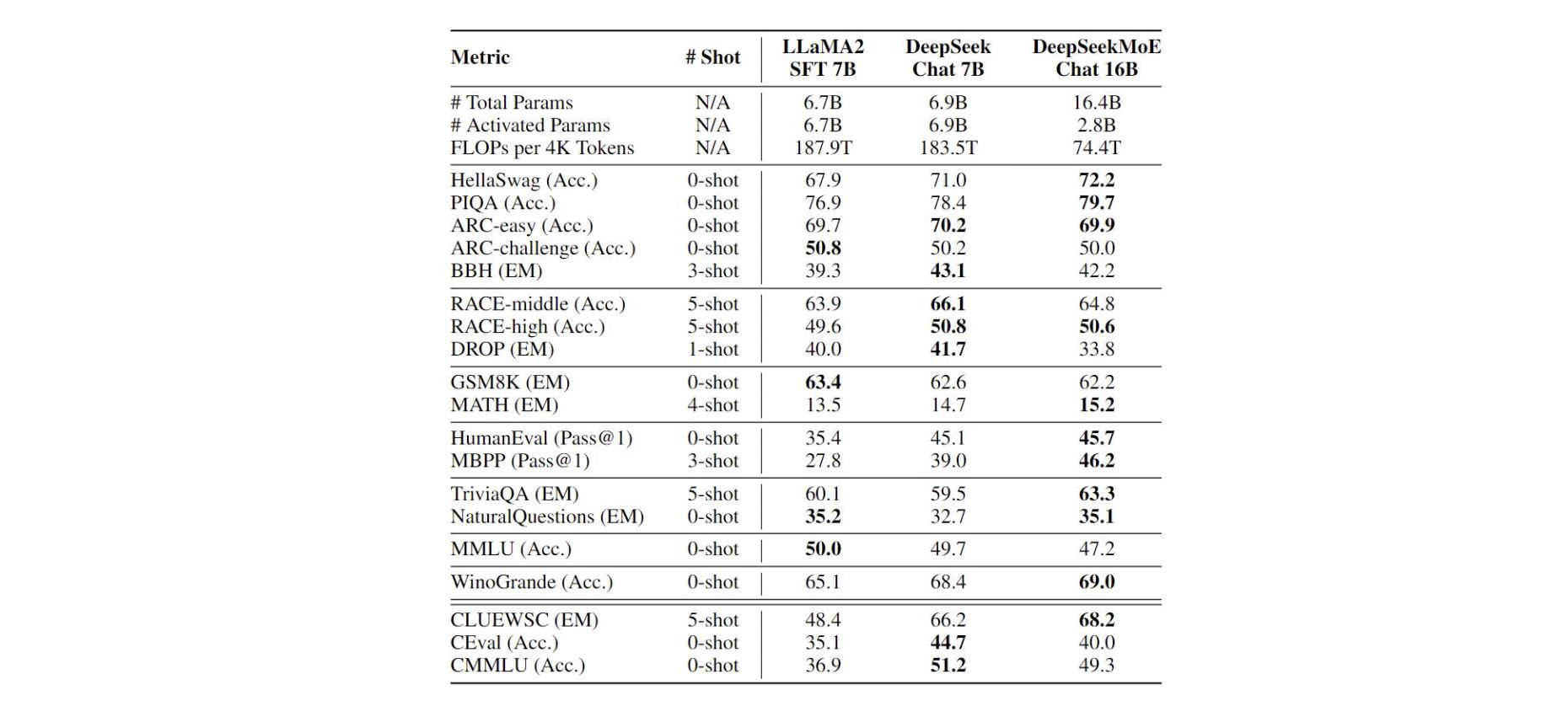
- 架构: DeepSeekMoE 16B 主要亮点在于 fine-grained expert segmentation 和 shared experts isolation.
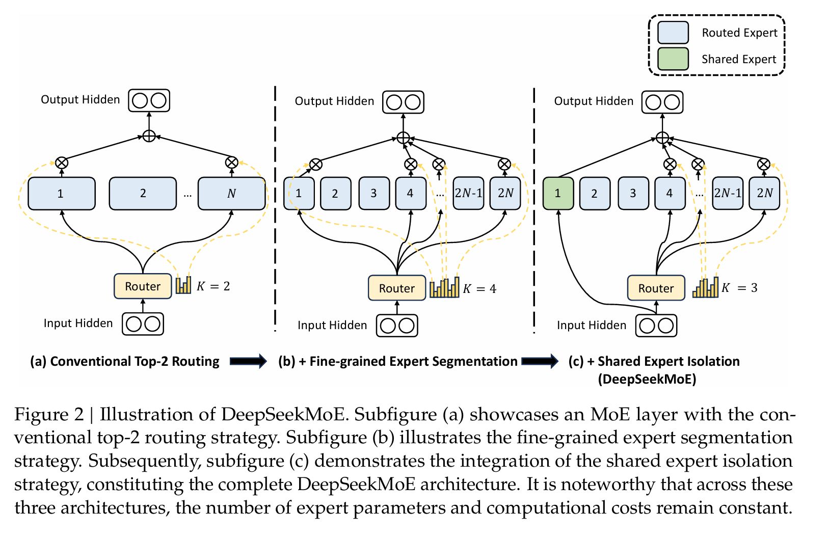
Fine-grained Expert Segmentation
如上图 B,DeepSeek-MoE 在减少了每个 expert FFN intermediate hidden dimension 的同时,增加激活的 expert 的数量,依次保证总体激活的 expert 的参数量一致。DeepSeekMoE 论文种认为,组合数量的提升,有利于 gate 更准确地选择 expert。
如当我们有 16 个 expert,然后选 top 2 进行推理时,activate expert 的组合数量有 种组合,但当将每个 expert 参数缩小 4 倍,expert 个数增加为 64 时,选取 top 8 进行推理时, activate expert 的组合书来给你就有 种。
Shared Expert Isolation
如上图 C,设立一部分 Shared Expert,每次推理的时候都会激活。
DeepSeek-V2
github, 论文链接,权重下载,huggingface 模型代码
DeepSeek-V2 文中推出了 DeepSeek-V2-Lite 与 DeepSeek-V2 一小一大 2 个版本。
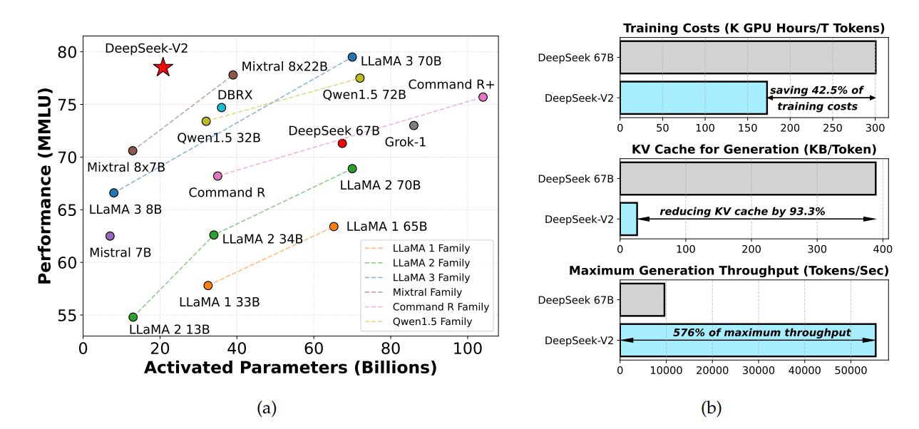
模型大小: DeepSeek-V2 整个模型有 236B 参数,其中推理激活参数为 21B。具体的架构参数可以查看:huggingface DeepSeek V2 config
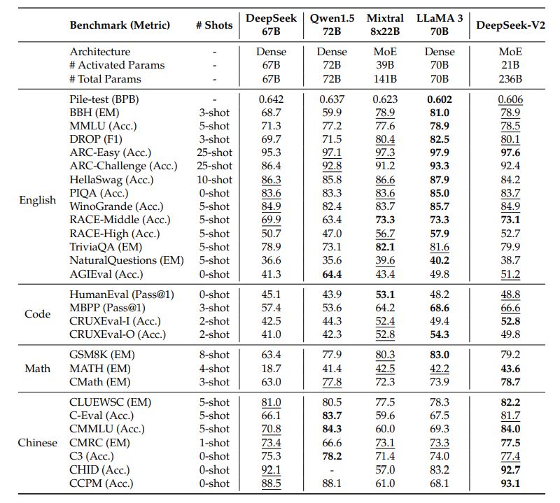
模型效果:
推理速度:
DeepSeek V2 首先对模型进行了 KV Cache 量化,将参数转换为了 FP8。在单机 8 卡 H800 的节点上部署 DeepSeek-V2,可以达到约 50K tokens/秒 的吞吐量
推理效果,中文水平更强一些,英文水平于 Mixtral 8*22B 有的一比:
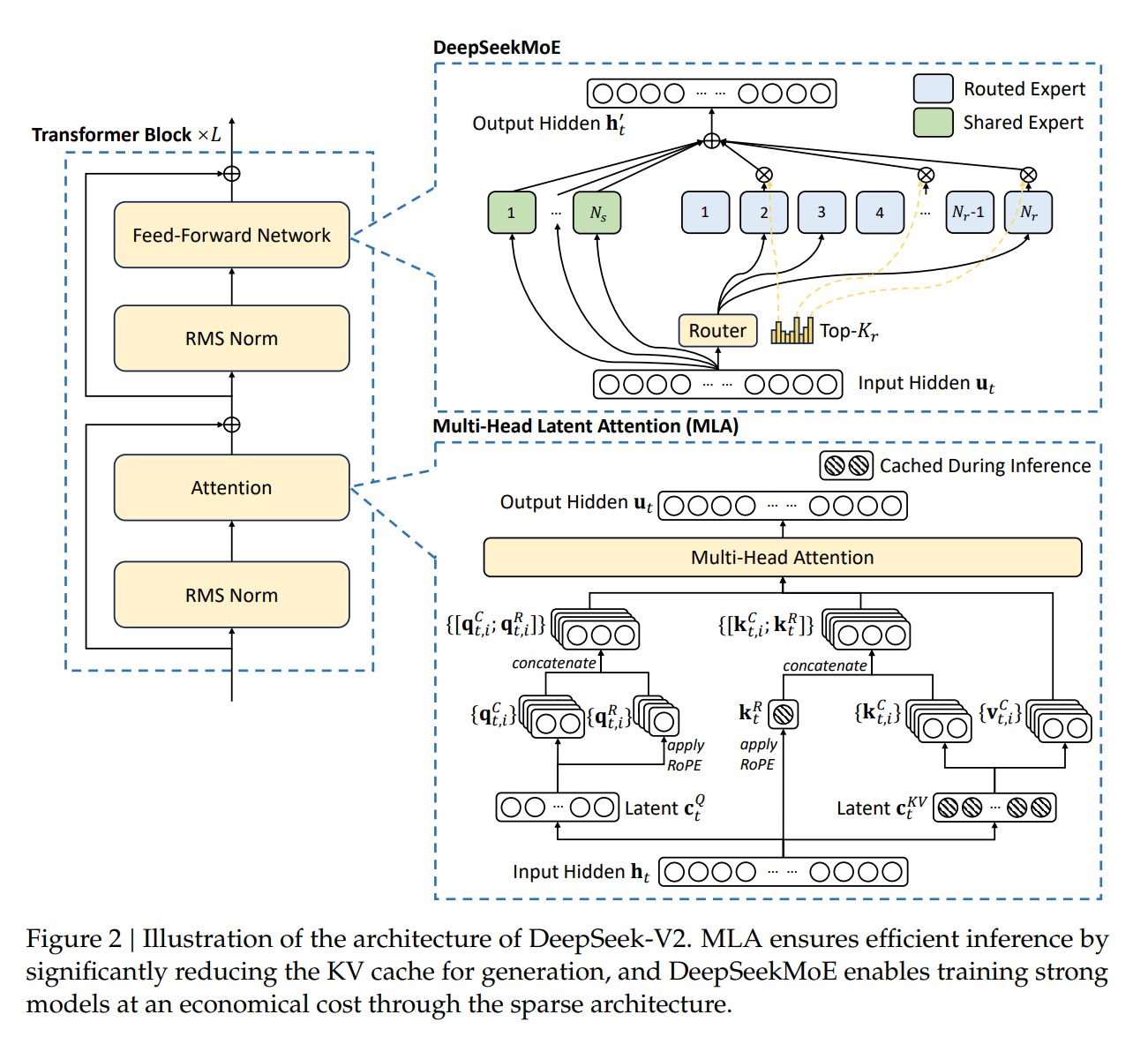
- 模型架构重点 :其中,架构采用了 MLA 取代 MHA,同时 MOE 架构采用了 DeepSeekMoE 的 fine-grained expert segmentation 和 shared experts isolation。整体的 DeepSeek Layer 架构如下:
对应到 huggingface 的实现为:
huggingface 代码
class DeepseekV2DecoderLayer(nn.Module):
    def __init__(self, config: DeepseekV2Config, layer_idx: int):
        super().__init__()
        self.hidden_size = config.hidden_size

        self.self_attn = ATTENTION_CLASSES[config._attn_implementation](
            config=config, layer_idx=layer_idx
        )

        self.mlp = (
            DeepseekV2MoE(config)
            if (
                config.n_routed_experts is not None
                and layer_idx >= config.first_k_dense_replace
                and layer_idx % config.moe_layer_freq == 0
            )
            else DeepseekV2MLP(config)
        )
        self.input_layernorm = DeepseekV2RMSNorm(
            config.hidden_size, eps=config.rms_norm_eps
        )
        self.post_attention_layernorm = DeepseekV2RMSNorm(
            config.hidden_size, eps=config.rms_norm_eps
        )

    def forward(
        self,
        hidden_states: torch.Tensor,
        attention_mask: Optional[torch.Tensor] = None,
        position_ids: Optional[torch.LongTensor] = None,
        past_key_value: Optional[Tuple[torch.Tensor]] = None,
        output_attentions: Optional[bool] = False,
        use_cache: Optional[bool] = False,
        **kwargs,
    ) -> Tuple[
        torch.FloatTensor, Optional[Tuple[torch.FloatTensor, torch.FloatTensor]]
    ]:
        if "padding_mask" in kwargs:
            warnings.warn(
                "Passing `padding_mask` is deprecated and will be removed in v4.37. Please make sure use `attention_mask` instead.`"
            )
        residual = hidden_states

        hidden_states = self.input_layernorm(hidden_states)

        # Self Attention
        hidden_states, self_attn_weights, present_key_value = self.self_attn(
            hidden_states=hidden_states,
            attention_mask=attention_mask,
            position_ids=position_ids,
            past_key_value=past_key_value,
            output_attentions=output_attentions,
            use_cache=use_cache,
            **kwargs,
        )
        hidden_states = residual + hidden_states

        # Fully Connected
        residual = hidden_states
        hidden_states = self.post_attention_layernorm(hidden_states)
        hidden_states = self.mlp(hidden_states)
        hidden_states = residual + hidden_states

        outputs = (hidden_states,)

        if output_attentions:
            outputs += (self_attn_weights,)

        if use_cache:
            outputs += (present_key_value,)

        return outputs
RMS norm
class DeepseekV2RMSNorm(nn.Module):
    def __init__(self, hidden_size, eps=1e-6):
        """
        DeepseekV2RMSNorm is equivalent to T5LayerNorm
        """
        super().__init__()
        self.weight = nn.Parameter(torch.ones(hidden_size))
        self.variance_epsilon = eps

    def forward(self, hidden_states):
        input_dtype = hidden_states.dtype
        hidden_states = hidden_states.to(torch.float32)
        variance = hidden_states.pow(2).mean(-1, keepdim=True)
        hidden_states = hidden_states * torch.rsqrt(variance + self.variance_epsilon)
        return self.weight * hidden_states.to(input_dtype)
- DeepSeekMoE
如上图展示的,DeepSeek-V2 同样采用了 DeepSeekMoE 的策略,其中有 2 个 shared experts , 160 个 routed experts(每次只激活 6 个)
- Multi-Head Latent Attention
DeepSeek-V2 中着重讲了这一部分的优化。
Low-Rank Key-Value Joint Compression
为了减少 KV cache,MLA 提出将 k, v 的计算方式变为:
其中, ,压缩后的维度 ; 为 kv_lora_rank, d_h 为 head_dim (包括 q_head_dim 和 v_head_dim)
q 的计算方法变为:
其中,; 为 q_lora_rank , d 为 hidden_size,; 为 q_head_dim, 为 num_head
因此,k,v 均从 进一步计算得来。在推理时候,传统 MHA 需要 cache ,但通过以上变化后,只需要 cache 即可。这样, 点积就变成了。
推理过程中,可以合并 ,以此达到减少 cache 同时,不会增加太多的计算量。
Decoupled Rotary Position Embedding
以上方案的一个问题是,不兼容 RoPE。由于 RoPE 的存在,
不再是单纯的 ,而是需要内积上相对位置矩阵 ,因此就无法简单得合并 。
MLA 采用了以下 decoupled RoPE 方案:
大概思路是,在原先的 qk 中,增加几个维度,用来注入 RoPE 位置信息,比较值得注意的是,k 新增加的维度 是所有 head 共享的。其中,, , 因此,q,k 的维度增加到了 。
更深入的 MLA 解读,可以参考:缓存与效果的极限拉扯:从 MHA、MQA、GQA 到 MLA 或 deepseek v2 原论文。
参考 huggingface 中 DeepseekV2Attention 的实现:
class DeepseekV2Attention(nn.Module):
    # 该笔记中省略了部分不重要的代码

    def __init__(self, config: DeepseekV2Config, layer_idx: Optional[int] = None):
        super().__init__()
        self.config = config
        self.layer_idx = layer_idx
        self.attention_dropout = config.attention_dropout
        self.hidden_size = config.hidden_size
        self.num_heads = config.num_attention_heads

        self.max_position_embeddings = config.max_position_embeddings
        self.rope_theta = config.rope_theta
        self.q_lora_rank = config.q_lora_rank
        self.qk_rope_head_dim = config.qk_rope_head_dim
        self.kv_lora_rank = config.kv_lora_rank
        self.v_head_dim = config.v_head_dim
        self.qk_nope_head_dim = config.qk_nope_head_dim
        self.q_head_dim = config.qk_nope_head_dim + config.qk_rope_head_dim

        self.is_causal = True

        self.q_a_proj = nn.Linear(
            self.hidden_size, config.q_lora_rank, bias=config.attention_bias
        )  # W^{DQ}; 其中 q_lora_rank = d'
        self.q_a_layernorm = DeepseekV2RMSNorm(config.q_lora_rank)
        self.q_b_proj = nn.Linear(
            config.q_lora_rank, self.num_heads * self.q_head_dim, bias=False  # 1536, 32 * (128+64)
        ) # W^{UQ}

        self.kv_a_proj_with_mqa = nn.Linear(
            self.hidden_size,  # 4096
            config.kv_lora_rank + config.qk_rope_head_dim,  # 512 + 64
            bias=config.attention_bias,
        )
        self.kv_a_layernorm = DeepseekV2RMSNorm(config.kv_lora_rank)
        self.kv_b_proj = nn.Linear(
            config.kv_lora_rank,
            self.num_heads
            * (self.q_head_dim - self.qk_rope_head_dim + self.v_head_dim),
            bias=False,
        )

        self.o_proj = nn.Linear(
            self.num_heads * self.v_head_dim,
            self.hidden_size,
            bias=config.attention_bias,
        )
        self._init_rope()

        self.softmax_scale = self.q_head_dim ** (-0.5)

    def _init_rope(self):
        self.rotary_emb = DeepseekV2RotaryEmbedding(
            self.qk_rope_head_dim,
            max_position_embeddings=self.max_position_embeddings,
            base=self.rope_theta,
        )

    def forward(
        self,
        hidden_states: torch.Tensor,
        attention_mask: Optional[torch.Tensor] = None,
        position_ids: Optional[torch.LongTensor] = None,
        past_key_value: Optional[Cache] = None,
        output_attentions: bool = False,
        use_cache: bool = False,
        **kwargs,
    ) -> Tuple[torch.Tensor, Optional[torch.Tensor], Optional[Tuple[torch.Tensor]]]:
        bsz, q_len, _ = hidden_states.size()

        q = self.q_b_proj(self.q_a_layernorm(self.q_a_proj(hidden_states)))  # q = W^{UQ}(norm(W^{DQ}h))  [batch size, len_seq, num_head * (128+64)]
        q = q.view(bsz, q_len, self.num_heads, self.q_head_dim).transpose(1, 2)
        q_nope, q_pe = torch.split(
            q, [self.qk_nope_head_dim, self.qk_rope_head_dim], dim=-1
        )
        # [bsz, num_head, q_len, 128]
        # [bsz, num_head, q_len, 64]

        compressed_kv = self.kv_a_proj_with_mqa(hidden_states)  # [bsz, len_seq, 512 + 64]

        compressed_kv, k_pe = torch.split(
            compressed_kv, [self.kv_lora_rank, self.qk_rope_head_dim], dim=-1
        )
        k_pe = k_pe.view(bsz, q_len, 1, self.qk_rope_head_dim).transpose(1, 2) # [bzs, 1, q_len, 64]
        kv = (
            self.kv_b_proj(self.kv_a_layernorm(compressed_kv))  # W^{UK}(norm(c_t^{KV}))
            .view(bsz, q_len, self.num_heads, self.qk_nope_head_dim + self.v_head_dim)
            .transpose(1, 2)
        )  # [bsz, num_head, q_len, 128 + 128]

        k_nope, value_states = torch.split(
            kv, [self.qk_nope_head_dim, self.v_head_dim], dim=-1
        )
        kv_seq_len = value_states.shape[-2]

        cos, sin = self.rotary_emb(value_states, seq_len=kv_seq_len)

        # 应用 decouple ROPE 方案
        q_pe, k_pe = apply_rotary_pos_emb(q_pe, k_pe, cos, sin, position_ids)

        query_states = k_pe.new_empty(bsz, self.num_heads, q_len, self.q_head_dim)
        query_states[:, :, :, : self.qk_nope_head_dim] = q_nope
        query_states[:, :, :, self.qk_nope_head_dim :] = q_pe

        key_states = k_pe.new_empty(bsz, self.num_heads, q_len, self.q_head_dim)
        key_states[:, :, :, : self.qk_nope_head_dim] = k_nope
        key_states[:, :, :, self.qk_nope_head_dim :] = k_pe

        attn_weights = (
            torch.matmul(query_states, key_states.transpose(2, 3)) * self.softmax_scale
        )

        # upcast attention to fp32
        attn_weights = nn.functional.softmax(
            attn_weights, dim=-1, dtype=torch.float32
        ).to(query_states.dtype)
        attn_weights = nn.functional.dropout(
            attn_weights, p=self.attention_dropout, training=self.training
        )
        attn_output = torch.matmul(attn_weights, value_states)

        attn_output = attn_output.transpose(1, 2).contiguous()

        attn_output = attn_output.reshape(bsz, q_len, self.num_heads * self.v_head_dim)

        attn_output = self.o_proj(attn_output)

        return attn_output, attn_weights, past_key_value
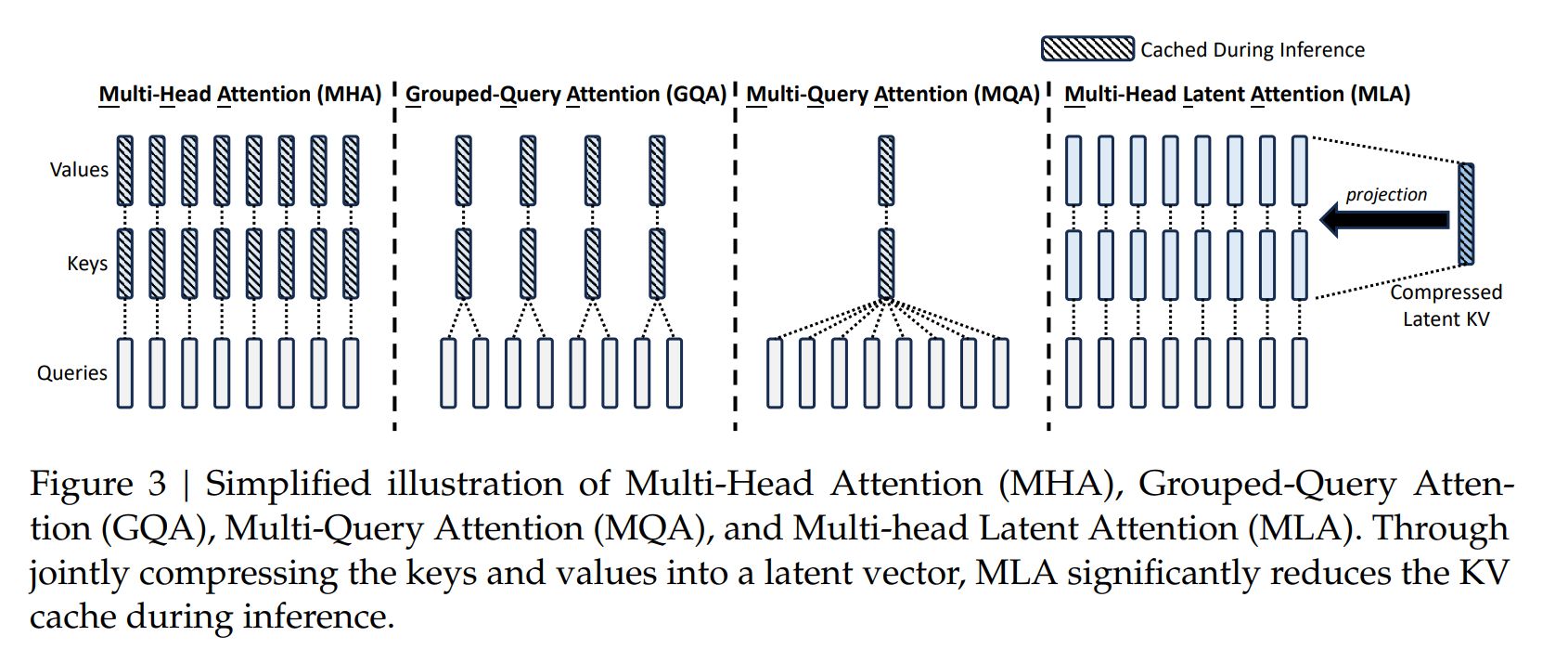
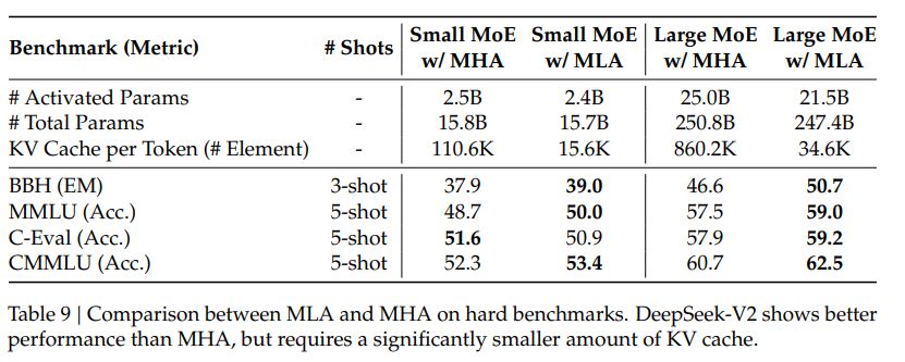
文中给出了 MLA 与 MHA, GQA 的效果对比:
MLA 的 KV 的 cache 数量比 MHA, GQA 少了不少。
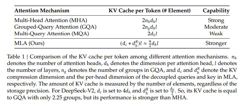
MLA KV cache 比 MHA 小的同时,效果也不会太差。
Auxiliary Loss for Load Balance
Deepseek V2 再模型训练时候,对 loss 进行了处理,以确保所有的 expert 都能得到合理的训练。假设 为 FFN 的输入,那么 FFN 的输出计算公式如下:
其中 和 为 shared 和 routed expert 数量, 或 为第 i 个 expert; 为激活的 routed expert 的数量; 为 gate value;
训练 loss 主要分为下面几个部分:
- Expert level Balance Loss:
其中 为超参, 为当前 token 的数量;当 routed expert 选择不平衡,有某个 routed expert 经常被选的时候, 会升高;
- Device-Level Balance Loss
Device-Level Balance Loss 的形式与 expert-level Balance Loss 相似,用于调整设备级别的平衡损失,以确保不同设备之间的计算负载均衡。在 DeepSeek-V2 的训练过程中,所有 routed expert 被划分为 D 组 ,并将每一组部署到单独的一台设备上。设备级别的平衡损失计算如下:
其中 为超参;
- Communication Balance Loss
Communication Balance Loss 用以确保每个设备的通信负载均衡。虽然设备限制路由机制保证了每个设备的发送通信量有上限,但如果某个设备接收的 token 比其他设备多,实际通信效率也会受到影响。为了缓解这一问题,deepseek 训练时采用了 Communication Balance Loss 计算如下:
其中, 为超参。设备限制路由机制的原则是确保每个设备最多向其他设备传输 MT 个 hidden state。同时,引入通信平衡损失以鼓励每个设备从其他设备接收大约 MT 个 hidden state。
除了以上几个 loss 外,Deepseek 再训练时也采用了 Token-Dropping Strategy。参考这个 issue,Deepseek-V3 中似乎没有采取该策略。
- 预训练: 相比于 DeepSeek 67B,DeepSeek-V2 训练集中有更多的中文数据,同时 DeepSeek V2 对数据过滤算法进行了改进,包括筛除有争议的内容等;DeepSeek V2 使用于 DeepSeek 67B 同样的 tokenizer,vocab size 为 100k,预训练语料约有 8.1T tokens,其中中文比英文多了 12%。整个预训练花费了 172.8K GPU hours 的算力。
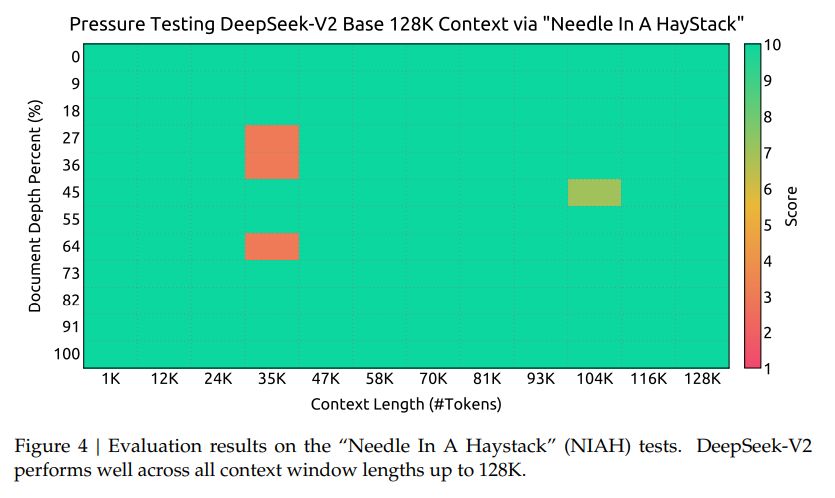
- 超长上下文: 在适配了 Yarn 之后,额外在 32k 的数据集上训练了 1000 steps,batch size 为 576。文中表示,尽管是在 32K 数据集上训练,但在 128K 的大海捞针测试中,模型表现也不错:
- SFT :在包含了 1.5M 组训练实例的数据集上,微调了 2 个 epoch。
- RLHF: 采用了 GRPO 来节省 RL 训练的成本,主要是将 PPO 过程中的 advantage 替换成了 ,因此在 RLHF 过程中就不需要 Value model 了。具体算法如下:
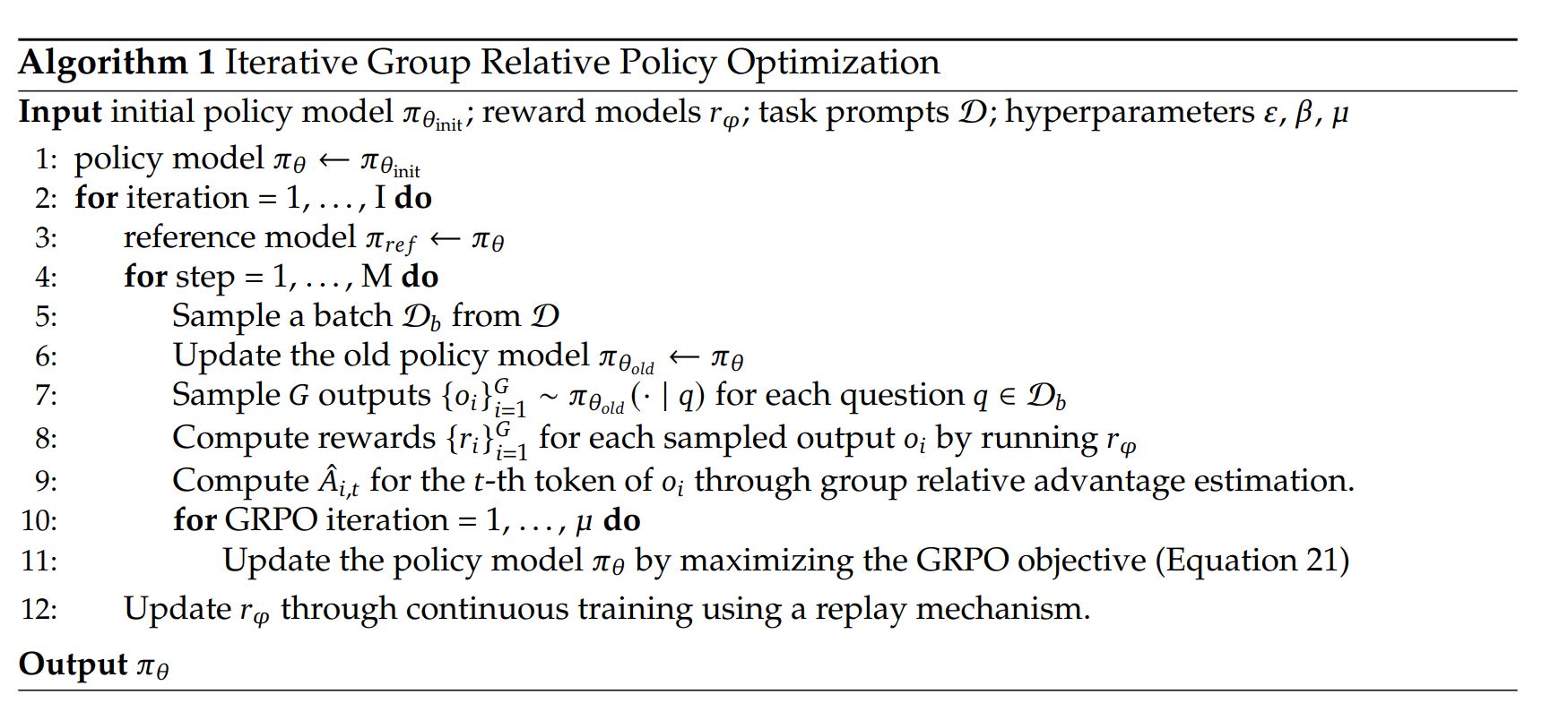
在 RLHF 训练过程中,采取了 2 阶段训练。首先进行了 reasoning alignment,而后进行 human preference alignment。
- Inference Efficiency: Deepseek V2 采用了一些策略来提高推理性能
- 参数转化为 FP8
- KV Cache 量化
部署了 Deepseek V2 MOE 后,再 1 台 H800 * 8 上可以实现 50K 每秒的 token 吞吐量。
DeepSeek V2 中提出的一些讨论
- SFT 数据量与质量
- 实验表明,低于 1 万条 SFT 数据会导致 IFEval 基准性能大幅下降。
- 随模型规模增大,所需数据量会减小,但仍需足够数据以掌握特定技能。
- 高质量的 SFT 数据对写作和开放式问答任务尤为重要。
- 对齐成本(Alignment Tax)
- RLHF 可显著提升开放式生成任务表现,但可能削弱 BBH 等标准基准性能。
- 通过精细化数据处理和改进训练策略,实现两者间的可接受权衡。
- 如何在保持整体性能的前提下完成偏好对齐,值得进一步研究。
- 在线强化学习优势
- 实验发现在线 RL 明显优于离线 RL,因此为 DeepSeek-V2 构建了在线 RL 框架。
- 在线/离线偏好对齐效果或因场景不同而异,后续需进行更全面对比。
更多训练细节欢迎参考 DeepSeek-V2 论文
Deepseek V3
DeepSeek-V3 Technical Report, huggingface 空间,Insights into DeepSeek-V3: Scaling Challenges and Reflections on Hardware for AI Architectures
架构
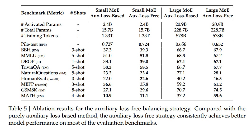
- 基础架构与 DeepSeek-V2 差不多,采用了 DeepSeek-v2 的 MLA 和 DeepSeekMOE,不同于 DeepSeek-V2 的是,采用了 auxiliary-loss-free load banlancing strategy。
- auxiliary-loss-free load banlancing strategy 在选择 expert 的计算过程中,加入了参数
论文中也给出了对比数据
- 提出了 Multi Token Prediction 目标
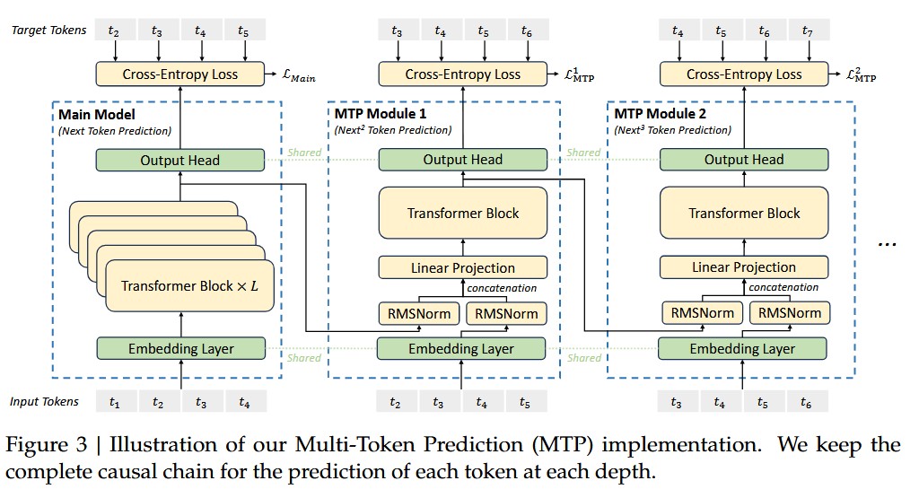
如上图所示,再训练时候,采用多个 MTP Module 对后几个 token 进行预测,第 k 个 MTP module 预测第 个开始的 token。如上图,假设整个序列有 T 个 token,那么 MTP Module 1 开始就预测第 3 到 T 个 token。 MTP Module 2 开始就预测第 4 到 T 个 token。
额外的优化目标为各个 MTP Module 的 cross entropy loss 平均; 为超参;
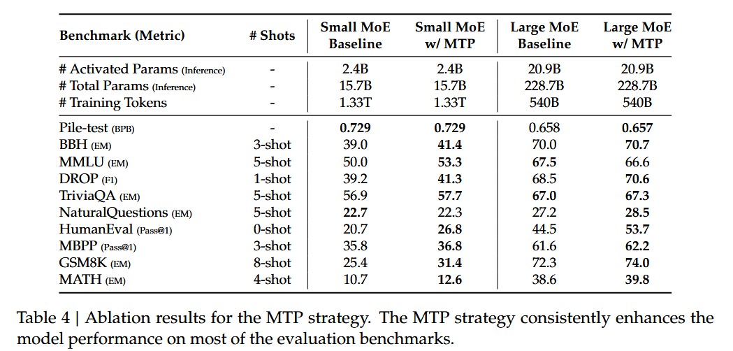
论文中也给出了 MTP 的对比测试
训练策略
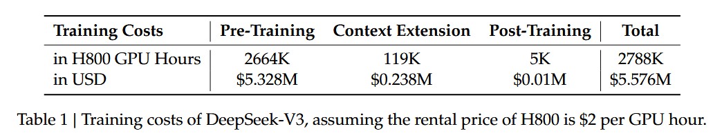
Deepseek V3 在 2048 个 H800 上训练。每个节点有 8 个 H800 GPU,通过 NVLink 和 NVSwitch 链接。节点接通信采用 InfiniBand。一些特殊的训练策略:
- 采用 DualPipe
- 开发了高效的 cross-node all-to-all communication kernel 来充分调用 IB 和 NVLink 的带宽,以及节约用于通信的 Streaming Multiprocessors 资源。
- 通过一系列显存管理策略,无需 Tensor Parallelism (TP) 的前提下即可完成 DeepSeek‑V3 的大规模训练。
- F8 混合精度训练,大部分的矩阵乘积操作都采用了 FP8 精度作为输入,输出 FP16 或者 FP32 。embedding,output head,MOE Gating 模块,norm 操作,attention 操作 都保留了原始的精度(BF16 或 FP32)
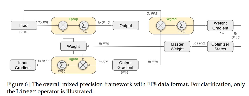
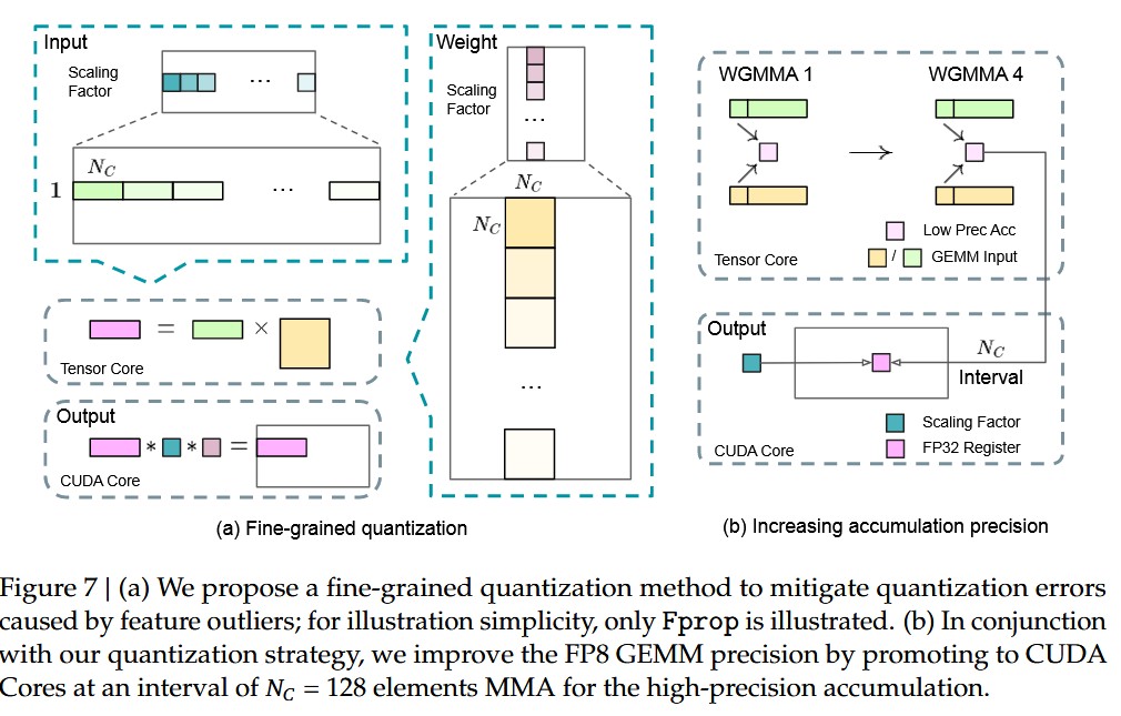
- Fine-Grained Quantization:
如下图,(该部分包含 GPT 解释)
缩放因子不要全局统一,而是 分组(fine-grained)计算 ,每组单独缩放。
- 激活(activations)
- 分组方式:以 1×128 的 tile 为单位(即“每个 token 的 128 个通道”作为一组)。
- 每个小组单独计算缩放因子并量化。
- 权重(weights)
- 分组方式:以 128×128 block 为单位(即 128 输入通道 × 128 输出通道)。
- 每个权重块单独缩放和量化。
- 累加策略:
- 在标准 FP8 GEMM 中,硬件只支持 整张量一个缩放因子 ;DeepSeek-V3 在 GEMM 的内积维度(K 维) 上插入了 per-group scaling factor 。每累加 一个 128 长度的片段(N_c = 128) ,就应用一次对应的缩放因子。
预训练
数据数量:14.8T,
V3 预训练过程中同样采用了 DeepSeekCoder-V2 16B 才用到的 FIM 策略,该策略将训练内容重新构造成了 prefix, suffix, middle 的模式,具体为 <|fim_begin|> fpre<|fim_hole|> fsuf<|fim_end|> fmiddle<|eos_token|> ,FIM 策略占用了 0.1 的训练比重。FIM 再 DeepSeekCoder-V2 当中,主要是用于训练模型挖空填充的能力,特别是针对代码补全的能力。
Long Context Extension
采用 YARN 额外训练了 2 个 1000 steps。分别将上下文窗口从 4k 提升到 32k,然后再提升到 128k。YARN 配置与 Deepseek-V2 一样
后训练
SFT -
包括了 1.5M 的训练实例
- 推理相关数据:采用 DeepSeek-R1 进行生成,并对生成数据进行了质量处理,避免冗长。
- 非推理相关数据:用 DeepSeek-V2.5 来生成回复,然后让人工标注员来验证数据的可靠性。
采用 5e-6 逐步下降到 1e-6 的学习率训练了 2 个 epoch。
Reinforcement learning - V3 采用了 rule-based reward Model 和 model-based RM 2 中不同的 reward model
Rule-based RM:比如对于一些数学题,一些 LeetCode 题目等有准确答案的 input,可以采用固定的方式来提供 feedback。
Model Based RM:
有唯一正确答案的题目 :由奖励模型(reward model)判断生成答案是否与预期的“真实值”匹配。
无唯一“标准答案”的题目(如创意写作) :奖励模型根据问题与对应回答给出反馈分数。
奖励模型来源
以 DeepSeek-V3 的 SFT(监督微调)检查点 为基础进行训练。
提高奖励模型可靠性的方法
构建的偏好数据不仅包含最终的奖励分数,还记录 产生该分数的推理链(chain-of-thought) 。
这样可以在具体任务中减少“奖励漏洞”(reward hacking)的风险,避免模型为了拿高分而走偏门。
Group Relative Policy Optimijzation: V3 同样采用了 GRPO
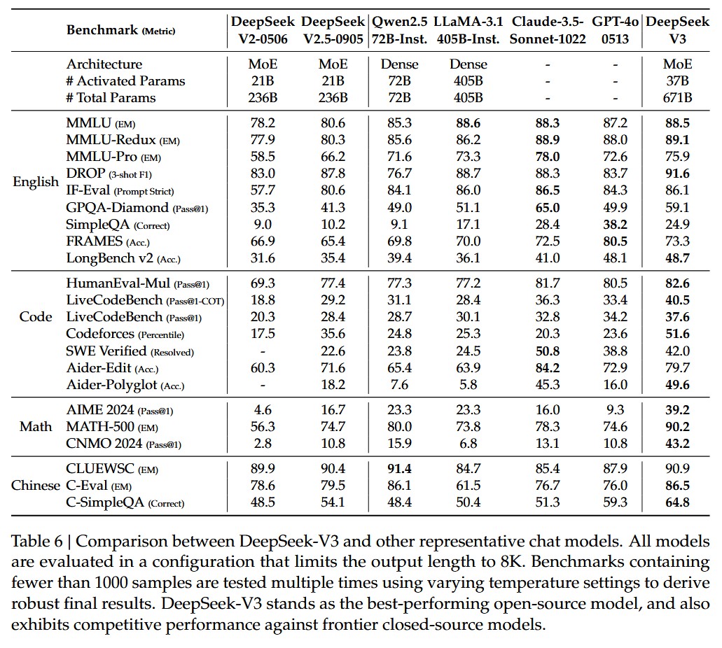
Evaluation
效果如下:
探索
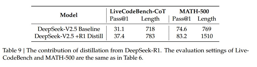
- 通过 DeepSeek-R1 蒸馏
通过 DeepSeek -R1 进行蒸馏,模型回答的质量会提高,但是回复长度也会边长。baseline 模型在短的 CoT 数据上面训练,而蒸馏版本则是完全使用 R1 生成的数据。
- self-rewarding
RL 阶段,采用了 constitutional AI 的策略,让模型进行自我反馈。 CAI 的步骤大概包括:
监督阶段(SL) :模型先回答一组提示;然后根据“宪法”由模型或反馈机制生成对回答的批评/建议;再让模型生成修正后的回答;然后将这些“修正”样本用来微调模型。
强化学习阶段(RL) :模型生成多个回答,然后使用一个偏好模型(preference model)来比较哪些回答更符合“宪法”原则;然后利用这些偏好信号进行 RL 优化。
整个过程中,人类控制更多是定义“宪法”原则,而不是每个回答都人工打标签。
- multi-token prediction evaluation
MTP 让模型在推理阶段能够一次 forward 预测 2 个 token ,并且 evaluation 阶段表明,第二个 token 的接受率在 85% - 90% 之间。当接受率高的时候, MTP 能够让 DeepSeek-V3 的推理速度提升 1.8 倍左右。
Deepseek R1
huggingface 空间: 链接
arxiv:https://arxiv.org/pdf/2501.12948
25 年 1 月左右出来的文章。
- 基于规则的 Reward
该方法采用了 2 种形式:
- Accuracy rewards:直接针对回复的正确性进行打分,比如一些 LeetCode 问题等具有标准答案的问题。
- Format rewards:要求模型在
<think></think>之间放入思考流程。
DeepSeek-R1-Zero 没有使用 ORM 或 PRM。
- DeepSeek-R1-Zero (64 乘 8 张 H800 GPU 训练 198 小时)

不依靠 SFT,完全依靠 RL 的模型,也能够实现理想的推理能力。7B,或 16B MOE 太小,无法通过单纯 RL 来获得显著提升。

DeepSeek-R1-Zero 在训练过程中的一个发现:模型的思考推理长度随着训练增加。一些复杂的能力也随着推理时间(test-time computation)的增加而涌现,比如反思能力 错误尝试 → 检查失败 → 改变策略 → 得到正确答案(模型重新审视并重新评估其先前的步骤,有时候模型会出现 “wait”, “mistake”, “however”, “but”, “retry”, “error”, “verify”, “wrong”, “evaluate”, and “check” 等词,但这些词的出现不一定就是 aha moment):

DeepSeek-R1-Zero 同时也有一些缺点,如回复难以理解,多种语言混用等问题。
- DeepSeek-R1 基于 DeepSeek-V3-Base 进行了以下的训练(80 小时,成本约$294K)
冷启动:
该阶段 SFT 采用 DeepSeek-R1-Zero 生成高质量的长 COT 回复,prompt 采用 few-shot,同时需要人为地对模型生成的结果进行后处理。
输出格式被定义成 |special_token|<reasoning_process>|special_token|<summary>,其中 <reasoning_process> 是 COT 部分。
基于推理的强化学习:
R1 采用了与 Zero 类似的强化学习策略,同时额外添加上了对语言一致性的对齐。虽然添加语言语种对齐会在一定程度上削弱模型效果,但是这为输出可读性带来的提升是巨大的。
Rejection Sampling 和 SFT
这一阶段用来训练模型在各个通用任务上的能力。
- Reasoning data:采用上一步训练完的模型,进行 Rejection Sampling。通过 DeepSeek-V3 进行评分。而后对数据集进行过滤,留下 600k 训练数据。
- Non-Reasoning data:部分数据采用了和 DeepSeek-V3 一样的 pipeline 来生成;一部分数据使用 DeepSeek-V3 + COT 来生成对应的回答;这部分数据有 200k 左右;
使用以上数据,进行了 2 轮 SFT。
额外的强化学习:
DS 发现该阶段模型利用 reward function 中的缺陷或偏差,从而获得很高的 reward 分数,但实际上并没有真正符合背后的人类意图。
用于提高模型 helpfulness,harmlessness,reasoning 等能力;
reasoning 相关数据,使用与 DeepSeek-R1-Zero 中提到的方式生成;
general data 采用了 reward model,整个 pipeline 基于 DeepSeek-V3 的 pipeline 搭建。
蒸馏:
论文提到把开源模型在上文提到的 800k SFT 数据上进行训练,能达到不错的效果。该部分只采用了 SFT。
如果采用 DeepSeek-R1-Zero 的训练方式训练小模型,那模型的效果不如蒸馏的:

DeepSeek-R1 的各个评测指标

附录中的一些发现
- Reward model 的 prompt 先让模型根据问题进行回答,然后再让模型把自己回复和案例做对比,最后才进行打分。
- STEM 数据集只会加入有标准答案,格式可读的数据。
- Zero 生成的 reasoning 过程不一定能够是可读的,V3 模型对于推理过程和总结部分进行优化。
- RL 训练时候,每 400 步更新一下 reference model。
- 通过 RL 训练 base model,使模型在推理时自然产生更长 CoT、自我验证和解法搜索,从而把一部分外部 inference-time search 能力内化到模型行为中。之前 TOT 有类似 BFS, DFS 的算法,如果单纯用 RL 再 countdown 上训练,思维过程中的确能看到 inference-time 在任务上使用 DFS 的能力。(参考 https://github.com/Jiayi-Pan/TinyZero.git )
- 关于对 nB 大小模型做 GRPO,reference model 约占 2n + forward buffer,rollout model 约 2n + KV cache + 比如 vLLM memory pool 等开销,actor model 约占 16n,与训练 LLM 开销差不多。
DeepSeek-R1 的一些开源复现:
- https://github.com/huggingface/open-r1